I’ve done my fair share of free online course-ware. Something that has always bothered me with SQL courses, is that they tend to only focus on writing query’s. Querying data only works you have data to work with. This chicken and the egg problem is easily addressed though. If you keep reading, I’ll show you how to install SQL server, load in data, create a dimension table, and read the data using R. The necessary files needed to follow along can be found on the Github Repo.

Downloading SQL Server

In order to set up a database on your local computer you first need to download SQL Server from here. The developer version has everything you’ll need and more importantly its free. Download the developer version and follow the prompts to install a Server locally. Additionally, you’re going to need to install SQL Server Management Studio, which can be found here. Once the installs are finished, fire up SMSS and you should see a splash screen. Select Database engine in the first box, your computer name should be the server name. Use windows authentication and you’re in.

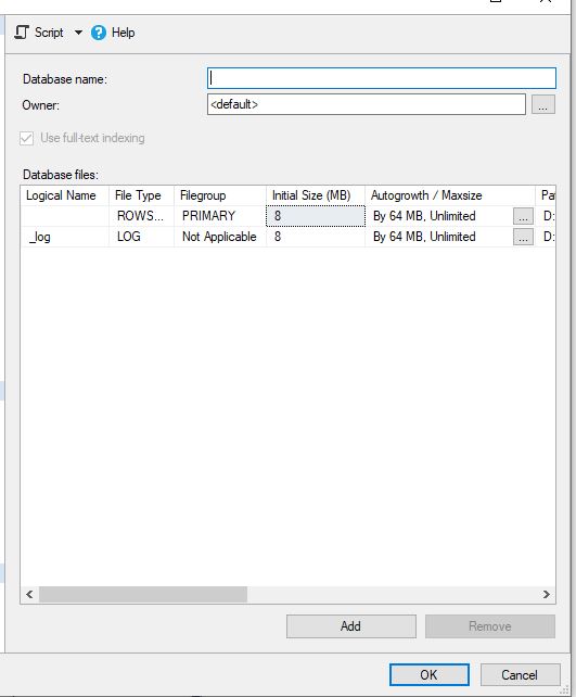
On the left you should have a tab that says object explorer. To create a new database, simply right click on the databases folder and click new database. The screen below should appear, enter the name you wish it to be called and then select okay.

Loading Data Into A Table

Step1: Go to the database you just created. Right click on the database -> task -> Import Data. The following import wizard should pop up.

Step 2: If you click next you’ll see a snapshot of what the data file looks like. If you need to skip some header columns you can click back. Click next.

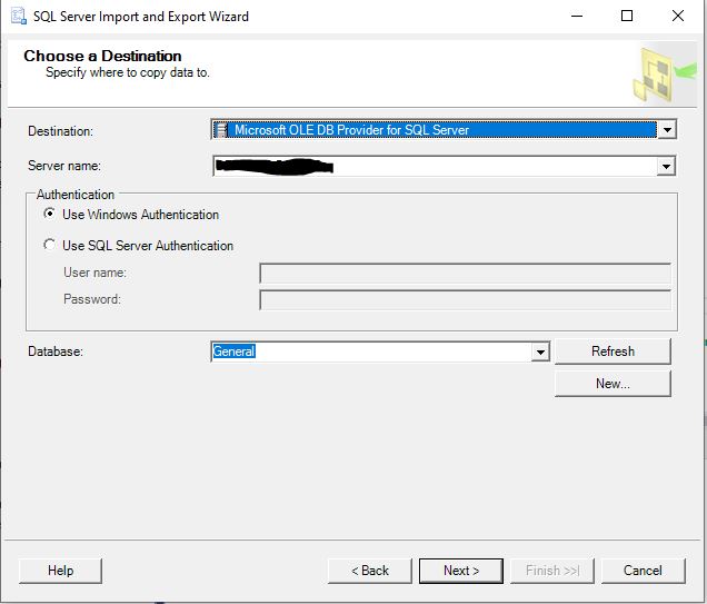
Step 3: Next you will be defining where to load the data to, Select the server and database that you have configured and press next.

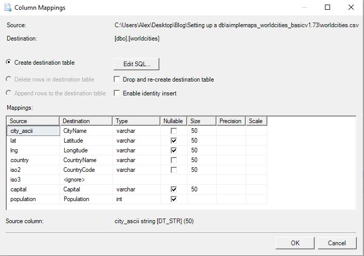
Step 4: Next we will be defining the mappings for the columns. Click Edit mappings and the following screen will pop up. In this menu you can determine column name, data type, and whether it can be null and data size limit.

Step 5: Click next, the import wizard detects some issues with population probably, set the global error and truncation rules to ignore and select next. Click next again and then finish and you should see this screen.

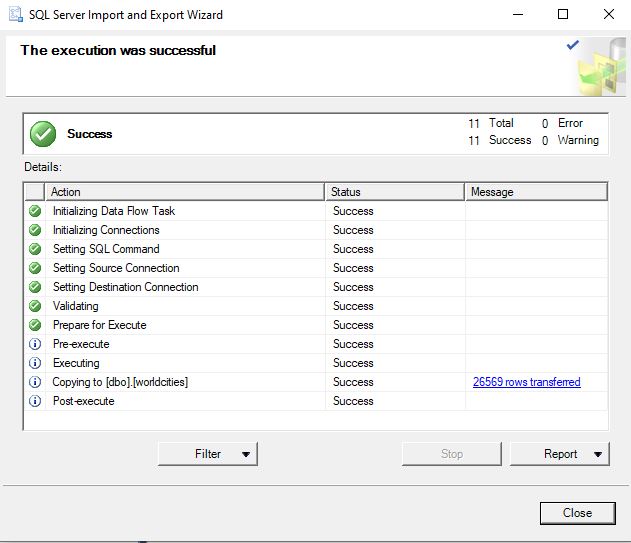
The data should be loaded into a data table now.

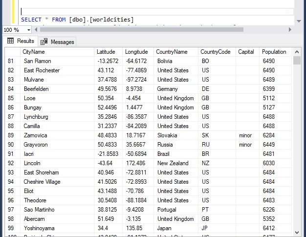
Basic Normalization

You may have noticed that the above snapshot has duplicate values in the Country Name and Code columns. While that isn’t necessarily a problem with this data set. Its poor form to not store data efficiently. The technical term for this process is “Normalization” and I wont go into depth on it here. This reference doc from Microsoft captures the broad strokes. Essentially you want to remove duplicate values and dependent values.

Since the Country name and code are duplicated throughout the data set, we can create a mapping table that links the country data back to the city data with a foreign key (integer). This integer key is much smaller as far as storage on the world cities table, and if we wanted to we could add more information to the countries table that doesn’t need to be on the cities table but would add value to the data set on a whole.

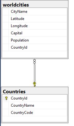
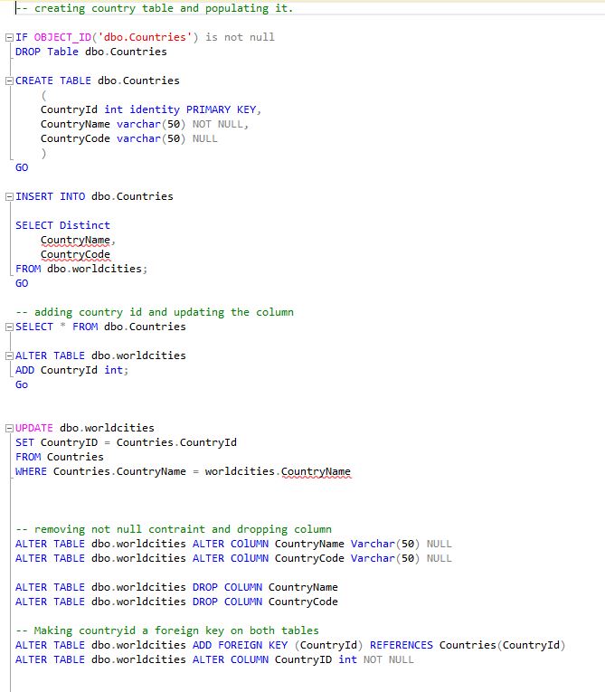
This is targeted end state. To get there, we need to populate a country table, link the two tables together through the id we create, and then remove the country name and code from the cities table. The SQL to do that is below. I have also attached the SQL code here.

Summary

Now you should have a database on your local computer with two tables of location data. Having the latitude and longitude mapped out for the Cities of the World will save a ton of time when performing any geographic analysis.

In order to get the full use out of our database an OBDC connection will need to be established. If you cant figure this out by yourself you’re not gonna make it.

Once the OBDC is set up we can easily access it with most analytical tools. I used R in this example, the full code is on the Github. My preference with R is to have the data as clean as possible before you even read it in, because arranging and cleaning data is R is sub-optimal.

Creating a map plot using this data is now quite simple, which justifies all the work we did in setting up a Database locally. To expand upon this, analysis projects will have overlapping data. Having these common datasets cleaned and ready to go saves a ton of time that can be put towards more rigorous analysis. If you found this post helpful please share and follow me on Twitter or LinkedIn to stay up to date on what I’m working on.